Seasonal Model

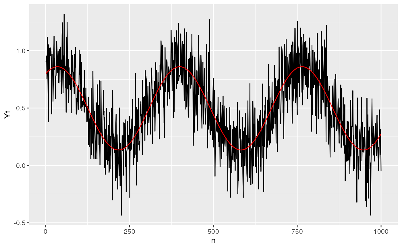
The seasonalModel class implements a seasonal regression model as a linear combination of sine and cosine functions. This model is designed to capture periodic effects in time series data, particularly for applications involving seasonal trends.

Details

The seasonal model is fitted using a specified formula, which allows for the inclusion of external regressors along with sine and cosine terms to model seasonal variations. The periodicity can be customized, and the model can be updated with new coefficients after the initial fit.

Note

Version 1.0.3

Public fields

extra_params

List to contain custom extra parameters.

control

List to contain custom control parameters.

Active bindings

period

Integer vector, periodicities of the seasonality.

order

Integer vector, number of combinations of sines and cosines.

omega

Integer, periodicity computed as \(\frac{2 \pi}{\text{period}}\).

coefficients

Named vector, model's parameters.

dcoefficients

Named vector, model's parameters for the differential with respect to n.

std.errors

Named vector, standard errors of the model's parameters.

coefs_names

Named vector, names of the model's parameters.

tidy

A tibble with estimated parameters and std. errors.

Methods

Public methods

• seasonalModel$new()

• seasonalModel$fit()

• seasonalModel$predict()

• seasonalModel$differential()

• seasonalModel$update()

• seasonalModel$update_coefs_names()

• seasonalModel$update_std.errors()

• seasonalModel$print()

• seasonalModel$clone()

---

Method new()

Initialize a seasonalModel object.

Usage

seasonalModel$new(formula, order = 1, period = 365)

Arguments

formula

formula, an object of class formula (or one that can be coerced to that class). It is a symbolic description of the model to be fitted and can be used to include or exclude the intercept or external regressors in data.

order

Integer, number of combinations of sines and cosines.

period

Integer, seasonality period. The default is 365.

---

Method fit()

Fit a seasonal model as a linear combination of sine and cosine functions and eventual external regressors specified in the formula. The external regressors used should have the same periodicity, i.e. not stochastic regressors are allowed.

Usage

seasonalModel$fit(data, ...)

Arguments

data

A data frame, list or environment (or object coercible by as.data.frame to a data frame) containing the variables in the model.

...

other parameters to be passed to the function lm.

---

Method predict()

Predict method for the class seasonalModel.

Usage

seasonalModel$predict(n, newdata)

Arguments

n

Integer vector, numbers of day of the year.

newdata

an optional data frame, list or environment (or object coercible by as.data.frame to a data frame) containing the variables in the model.

---

Method differential()

Compute the differential with respect to time (n).

Usage

seasonalModel$differential(n, newdata)

Arguments

n

Integer, number of day of the year.

newdata

an optional data frame, list or environment (or object coercible by as.data.frame to a data frame) containing the variables in the model.

---

Method update()

Update the parameters.

Usage

seasonalModel$update(coefficients)

Arguments

coefficients

Named vector, with new parameters, the names should match the names of the coefficients.

---

Method update_coefs_names()

Update the names of the parameters.

Usage

seasonalModel$update_coefs_names(coefs_names)

Arguments

coefs_names

Named vector, new parameters names, the names should match the names of the old coefficients.

---

Method update_std.errors()

Update the standard errors of the parameter.

Usage

seasonalModel$update_std.errors(std.errors)

Arguments

std.errors

Named vector with new standard errors, the names should match the names of the coefficients.

---

Method print()

Print method for the class seasonalModel.

Usage

seasonalModel$print()

---

Method clone()

The objects of this class are cloneable with this method.

Usage

seasonalModel$clone(deep = FALSE)

Arguments

deep

Whether to make a deep clone.

Examples

# Sample time series
n <- 1000
eps <- rnorm(n, sd = 0.2)
Yt <- 0.5 + 0.2 * sin(2*base::pi/365*c(1:n)) + 0.3 * cos(2*base::pi/365*c(1:n)) + eps

# Initialize the model
sm <- seasonalModel$new("Yt ~ 1", 1, 365)
# Fit the model
data = data.frame(Yt = Yt, n = 1:1000)
sm$fit(data = data)
data$Yt_hat <- sm$predict(n = data$n)
# Fitted parameters
sm$coefficients
#> intercept sin_1_365 cos_1_365 
#> 0.4974323 0.2044797 0.3000542 

# Plot the fitted data
library(ggplot2)
ggplot()+
geom_line(data = data, aes(n, Yt))+
geom_line(data = data, aes(n, Yt_hat), color = "red")